Abnormal Event Detection at 150 FPS in MATLAB

Authors: Cewu Lu, Jianping Shi, Jiaya Jia

PDF

Introduction

Difficulties in detecting abnormal events based on surveillance videos

• Hard to list all possible negative samples

Traditional method

• Normal patterns are learned from training

• And then the patterns are used to detect events deviated from this representation

Other methods

• Trajectories extracted from object-of-interest are used as normal patterns

• Learn normal low-level video feature distributions(exponential, multivariate Gaussian mixture, clustering)

• Graph model normal event representations which use co-occurrence patterns

• sparsity-based model(not fast enough for realtime processing due to the inherently intensive computation to build sparse representation)

Sparsity Based Abnormality Detection

• Sparsity: A general constraint to model normal event patterns as a linear combination of a set of basis atoms

• Computationally expensive

  $$min\|x-D\beta\|^2_2 \qquad s.t. \qquad \|\beta\|_0 \le s$$

  $\beta$ : parse coefficients

  $|x-D\beta|^2_2 $ :data fitting term

  $|\beta|_0$ : sparsity regulization term

  $s$ : parameter to control sparsity

  • abnormal pattern: large error result from $|x-D\beta|^2_2$

• Efficiency problem

  Adopting $min|x-D\beta|^2_2$ is time-consuming :

  • find the suitable basis vectors (with scale $s$) from the dictionary (with scale $q$) to represent testing data $x$

  • Search space is large ( $(^q_s)$ different combinations )

• Our contribution

  • Instead of coding sparsity by finding an $s$ basis combination from $D$ in $min|x-D\beta|^2_2$, we code it directly as a set of possible combinations of basis vectors

  • We only need to find the most suitable combination by evaluating the small-scale least square error

  

  • Freely selecting $s$ basis vectors from a total of $q$ vectors, the reconstructed structure could deviate from input due to the large freedom. However, in our method, each combination finds its corresponding input data

  • It reaches 140∼150 FPS using a desktop with 3.4GHz CPU and 8G memory in MATLAB 2012.

Methods

Learning Combinations on Training Data

• Preprocess

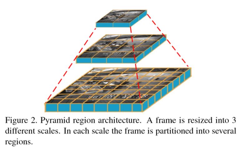
  • Resize each frame into different scales as “Sparse Reconstruction Cost for Abnormal Event Detection”

  • Uniformly partition each layer to a set of non-overlapping patches. All patches have the same size

  • Corresponding regions in 5 continuous frames are stacked together to form a spatial-temporal cube.

  • 

  This pyramid involves local information in fine-scale layers and more global structures in small-resolution ones.

  • With the spatial-temporal cubes, we compute 3D gradient features on each of them following “Anomaly Detection in Extremely Crowded Scenes Using Spatio-Temporal Motion Pattern Models”

  • Features are processed separately according to their spatial coordinates. Only features at the same spatial location in the video frames are used together for training and testing.

• Learning Combinations on Training Data

  • 3D gradient features in all frames gathered temporally for training are denoted as $X=\{x_1, x_2, ..., x_n\} \in R^{p*n}$. Each $x_i$ has $p$ features and there are $n$ $x_i$ in the $X$

  • Our goal is to find a sparse basis combination set $S=\{S_1, S_2, ..., S_K\}$ with each $S_i \in R^{p*s}$. Each $S_i$ combines $s$ dictionary basis vectors and each basis vector has $p$ features which correspond to the features in $x_i$. Each $S_i$ belongs to a closed, convex and bounded set, which ensures column-wise unit norm to prevent over-fitting

  • Reconstruction Error $t=min_{s,\gamma,\beta}\sum_{j=1}^n\sum_{i=1}^K\gamma_j^i\|x_j-S_i\beta_j^i\|_2^2 \quad s.t. \sum_{i=1}^K\gamma_j^i=1,\gamma_j^i=\{0,1\}$

  • Each $\gamma_j^i$ indicates whether or not the $i^{th}%$ combination $S_i$ is chosen for data $x_j$ and only one combination $S_i$ is selected for each $x_j$

  • $K$ must be small enough because a very large $K$ could possibly make the reconstruction error $t$ always close to zero(Don’t understand), even for abnormal events. However, we want the errors to be larger for abnormal events

• Optimization for Training

  • Problem : Reducing $K$ could increase reconstruction errors $t$. And it is not optimal to fix $K$ as well, as content may vary among videos

  • Solution : A maximum representation strategy. It automatically finds $K$ while not wildly increasing the reconstruction error $t$. In fact, error $t$ for each training feature is upper bounded in our method

  • Updated function

  $$t_j=\sum_{i=1}^K\gamma_j^i \{ \|x_j-S_i\beta_j^i \|_2^2 -\lambda \} \le 0,\quad s.t. \sum_{i=1}^K\gamma_j^i=1,\gamma_j^i=\{0,1\}$$
  • $\lambda :$ We obtain a set of combinations with a small $K$ by setting a reconstruction error upper bound $\lambda$ uniformly for each $S_i$. If $t_j$ is smaller than $\lambda$, the coding result is with good quality

• Algorithm

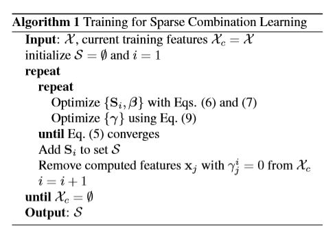
  • In each pass, we update only one combination, making it represent as many training data as possible

  • This process can quickly find the dominating combinations encoding important and most common features

  • Remaining training cube features that cannot be well represented by this combination are sent to the next round to gather residual maximum commonness

  • This process ends until all training data are computed and bounded

  • The size of combination $K$ reflects how informative the training data are

  • In each pass, we solve the equation above by interatively update ${S_s^i,\beta}$ and $\lambda$

    1. Update ${S_s^i,\beta}$ :
    $$L(\beta,S_i)=\sum_{j \in \Omega_c}\gamma_j^i \{ \|x_j-S_i\beta_j^i \|_2^2 \}$$ $$\beta_j^i=(S_i^TS_i)^{-1}S_i^Tx_j$$

    (Optimize $\beta$ while fixing $S_i$ for all $\gamma_j^i \neq 0$)

    $$S_i=\prod[S_i-\delta_t\bigtriangledown_{S_i}L(\beta,S_i)]$$

    ( Using block-coordinate descent( Online learning for matrix factorization and sparse coding and set $\delta = 1E-4$)

    1. Update $\gamma$ :
    $$\gamma_j^i = \left\{ \begin{aligned} 1 \quad & if \quad \|x_j-S_i\beta_j^i \|_2^2 < \lambda ; \\ 0 \quad & otherwise ;\\ \end{aligned} \right .$$

  

  The algorithm is controlled by $\lambda$, Reducing it could lead to a larger $K$

• Testing

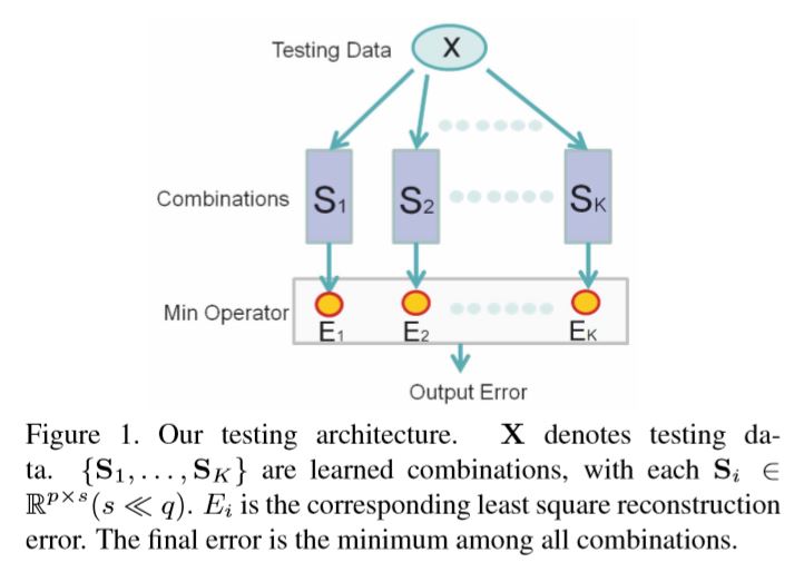
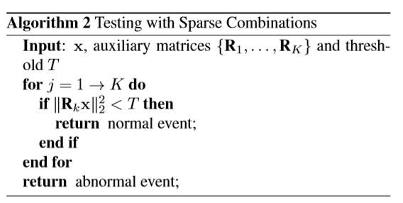
  • With the learned sparse combinations $S = {S_1, …, S_K}$, in the testing phase with new data $x$, we checki f there exists a combination in $S$ fitting the $\lambda$. It can be quickly achieved by checking the least square error for each $S_i$
  $$min_{\beta^i}\|x_j-S_i\beta_j^i \|_2^2 \quad \forall i= 1, ..., K$$
  • optimal solution :
  $$\hat{\beta^i}=(S_i^TS_i)^{-1}S_i^Tx$$
  • Reconstruction error in $S_i$ :
  $$\|x_j-S_i\beta_j^i \|_2^2 = \|((S_i^TS_i)^{-1}S_i^T-I_p)x\|_2^2=\|R_ix\|_2^2$$

  

  • It is noted that the first a few dominating combinations represent the largest number of normal event features.

  • Easy to parallel to achieve $O(1)$ complexity

  • Average combination checking ratio $= \frac{The\ number\ of\ combinations\ checked}{The\ total\ number\ K}$

• Relation to Subspace Clustering

Experiments

System Settings

• Resize each frame to 3 scales: $20*20, 30*40, 120*160$ pixels respectively

• Uniformly partition each layer to a set of non-overlapping 10×10 patches (totaly 208 sub-regions for each frame $\frac{20*30+30*40+120*160}{10*10}=208$ )

  

• Corresponding sub-regions in 5 continuous frames are stacked together to form a spatial temporal cube with resolution $10*10*5$

• Compute 3D gradient features on each cube and concatenate them into a 1500-dimension feature vector

• Reduce the feature vector to 100 dimensions via PCA

• Normalize the reduced feature vector to make it mean 0 and variance 1

• For each frame, we compute an abnormal indicator $V$ by summing the number of cubes in each scale with weights

  $$V=\sum_{i=1}^n 2^{n-i}v_i$$

  $v_i$ : the number of abnormal cubes in scale $i$, the top scale is with index $1$ while the bottom one is with $n$.

Verification of Sparse Combinations

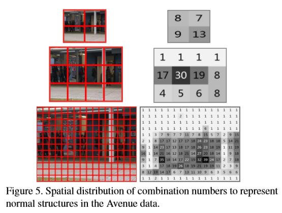
• Each video contains 208 regions and each region correspond to a cube and there are 6000-12000 features in each sube

• The features are used to verify the combination model. The number of combinations for each region is $K$

  The mean of $K$ is 9.75 and variance is 10.62, indicating 10 combinations are generally enough in our model

说人话

• 假设有一个学习好的$D\in R^{p \times q}$, 稀疏系数$\alpha_i$的0范数小于等于$s$

  也就是每个样本$x_i$最多能用$s$个字典基来表达。因为要稀疏，显然有$s « q$

  对于每个$x_i$，测试时都要从$q$个字典基中找出$s$个来表示，要求使得损失函数最小。

  因此这种测试方式很花时间（每次都在求解一个优化问题）

• 这篇文章主要解决了效率问题，提出了新的测试方式（训练$D$的方式也随之改变）：

  预先训练好$K$个稀疏表达$S_1 … S_K$，每个表达$S_i$都由$D$中的$s$个字典基组成

  测试时，将$x_i$与每个$S_i$计算得到损失函数，选择损失最小的$S_i$即可

• 重点在于得到$K$个$S_i$：

  设置一个损失函数上限$\lambda$，低于这个上限就认为编码质量好

  每个周期更新一个$S_i$，使其遍历在之前的周期还未被很好表达的$x_i$（也就是说，不论用什么已获得的$S_i$，该$x_i$的损失函数都超过$\lambda$）。

  对于每个周期未被很好表达的$x_i$，都留到下一个周期通过新的$S_i$来表达。如此循环直到所有$x_i$都可以被很好的表达。

• 在每次循环得到新的$S_i$的过程中：

  目标函数为： $min_{S_i,\gamma,\beta}\sum_{i=1}^K\gamma_j^i ( \|x_j-S_i\beta_j^i \|_2^2 -\lambda ),\quad s.t. \sum_{i=1}^K\gamma_j^i=1,\gamma_j^i=\{0,1\}$

  分 2 步解决这个问题

  • 更新$S_s^i,\beta$ :

    (更新 $\beta$ 时固定 $S_i$ 并且所有 $\gamma_j^i \neq 0$)

    1. $$\beta_j^i=(S_i^TS_i)^{-1}S_i^Tx_j$$
    2. $$S_i=\prod[S_i-\delta_t\bigtriangledown_{S_i}L(\beta,S_i)]$$ $$\delta = 1E-4$$

    详情请见Online Learning for Matrix Factorization and Sparse Coding中的算法1和算法2

    

  • 更新$\gamma$ :

    $$\gamma_j^i = \left\{ \begin{aligned} 1 \quad & if \quad \|x_j-S_i\beta_j^i \|_2^2 < \lambda ; \\ 0 \quad & otherwise ;\\ \end{aligned} \right .$$

• 测试

  对于目标函数： $min_{\beta^i}\|x_j-S_i\beta_j^i \|_2^2 \quad \forall i= 1, ..., K$

  最优解为: $\hat{\beta^i}=(S_i^TS_i)^{-1}S_i^Tx$

  损失函数可化为： $\|x_j-S_i\beta_j^i \|_2^2 = \|((S_i^TS_i)^{-1}S_i^T-I_p)x\|_2^2=\|R_ix\|_2^2$

  

---

• ← Previous Post
• Next Post →