Online Learning for Matrix Factorization and Sparse Coding

Authors: Julien Mairal, Francis Bach, Jean Ponce, Guillermo Sapiro
PDF

1. Introduction

Linear decompositon of a matrix using learned dictionary instead of pre-defined one

Usage:

• low-level: image denoising, texture synthesis, audio processing

• high-level: image classification

Differences between maxtrix factorization and PCA:

• It doesn’t impose that the basis vector to be orthogonal

• Allowing more flexibility to adapt the representation to the data

Variants matrix factorization problem:

• Non-negtive matrix factorization

• Sparse PCA

2. Problem Statement

• Optimize the empirical cost function:

  $$f_n(D) = \frac{1}{n}\sum_{i=1}^n l (x_i,D)$$

  • $D\in R^{m * k}$ :dictionary

  • $m < < n$: feature nums less than sample nums

  • $k < < n$: atom nums of dictoinary less than sample nums

  • $k > m$: Overcomplete dictionary: atoms more than feature nums

• $l_1$ sparse coding problem (basis pursuit):

$$l_1(x,D) = min\frac{1}{2}{\|x-D\alpha\|}_2^2+\lambda\|\alpha\|_1 \quad s.t. \quad \alpha \in R^k$$

• Disadvantage:

  There is no direct analytic link between the value of $\lambda$ and the corresponding effective sparsity $|\alpha|_0$

• Solution:

  To prevent $D$ from having arbitrarily large values (which would lead to arbitrarily small values of $\alpha$), it is common to constrain its columns $d_1, . . . ,d_k$ to have an $l_2-norm$ less than or equal to 1

  $$C = \{D \in R^{m * k}\quad s.t. \quad \forall j=1, ... ,k \quad d_j^Td_j \le 1\}$$

  It’s a joint optimization problem with respet to $D$ and $\alpha=[\alpha_1, …, \alpha_k] \in R^{k * n}$, which is not jointly convex but convex with respect to each of the two variables $D$ and $\alpha$ when the other one is fixed

• Optimization method:

  • Alternate between the two variables, minimizing over one while keeping the other one fixed

  • Since the computation of $\alpha$ dominates the cost of each iteration in this block-coordinate descent approach, a second-order optimization technique can be used to accurately estimate $D$ at each step when $\alpha$ is fixed

• Stochastic gradient

  Its rate of convergence is very poor in conventional optimization terms, may in fact in certain settings to be faster in reaching a solution with low expected cost than second-order batch

• Dictionary learning:

  The classical projected first-order projected stochastic gradient descent consists of a sequence of updates of $D$

  $$D_t = \prod [{D_{t-1}-\delta_t \nabla_C l(x_t,D_{t-1})}]$$

  • $\nabla_C: \quad$ Orthogonal projector onto $C$

  • $x_t: \quad$ i.i.d samples obtained by cycling on a randomly permuted training set

  • $\delta_t: \quad$ learning rate(good results are obtained using $\delta_t = \frac{a}{t+b}$ where $a$ and $b$ are chosen depended on the training data)

3. Online Dictionary Learning

3.1 Algorithm Outline

• Assuming that the training set is composed of i.i.d. samples

• $$f_t(D) = \frac{1}{t}\sum_{i=1}^t l (x_i,D)$$

  and

  $$\hat{f_t}(D) = \frac{1}{t}\sum_{i=1}^t(\frac{1}{2}\|x_i-D\alpha_i\|_2^2+\lambda\|\alpha_i\|_1)$$

  converge almost surely to the same limit, and thus that $\hat{f_t}$ acts as a surrogate for $f_t$

• Since $\hat{f_t}$ is close to $\hat{f_{t-1}}$ for large values of $t$, so are $D_t$ and $D_{t−1}$, use $D_{t−1}$ as warm restart for computing $D_t$ can acceerate this algorithm

3.2 Sparse Coding

This is a $l_1$ regularized linear least-squares problem :

$$l_1(x,D) = min\frac{1}{2}{\|x-D\alpha\|}_2^2+\lambda\|\alpha\|_1 \quad s.t. \quad \alpha \in R^k$$

• Traditional method (Coordinate descent with soft thresholding)

  • It is efficient when the columns of the dictionary are low correlated

  • Problem: The columns of learned dictionaries are in general highly correlated, which make this method rather slow

• New method (LARS-Lasso algorithm)

  • With an efficient Cholesky-based implementation, it is at least as fast as the one above

  • It provides the solution with a higher accuracy and being more robust since it does not require an arbitrary stopping criterion

3.3 Dictionary Update

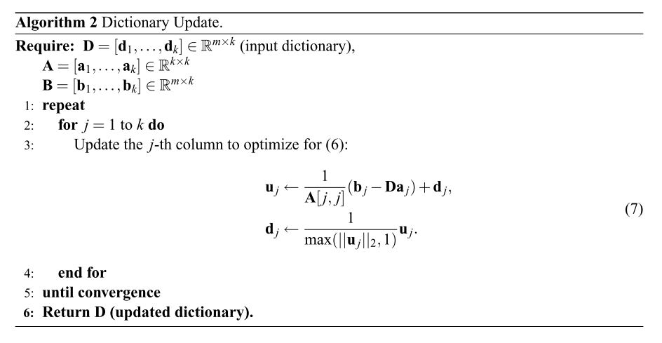
• The procedure does not require to store all the vectors $x_i$ and $\alpha_i$, but only $A_t$ and $B_t$

• Sequentially updates each column of $D$

• Orthogonal projection on to $C$(the constraint set)

• In practice, the matrix $A_t$ are often concentrated on the diagonal, which makes the block-coordinate descent more efficient

3.4 Optimizing the Algorithm

• 3.4.1 Handling fixed-size data sets

  • Problem: When the data sets are predefined and have finite size, the same data points may be examined several times

  • Solution: When the training set is small enough, it is possible to further speed up convergence:

    If the sample $x$ has been drawn from the data sets twice in the iteration $t_0$ and $t$, we will replace $\alpha_{t_0}$ by $\alpha_t$ in $A_t$ and $B_t$, that is

    $$A_t = A_{t-1} + \alpha_t\alpha_t^T - \alpha_{t_0}\alpha_{t_0}^T$$ $$B_t = B_{t-1} + x_t\alpha_t^T - x_t\alpha_{t_0}^T$$

    In this setting, we need to store $\alpha_i$ in every iteration and it’s impractical

    However, we can sovle this by removing the information from $A_t$ and $B_t$ that is older than two epochs(cycles through the data)

• 3.4.2 Scaling te past data

  • Problem: At each iteration, the “new” information $\alpha_t$ that is added to $A_t$ and $B_t$ has the same weight as the “old” one

  • Solution: Rescaling the “old” information so that newer coefficients $\alpha_t$ have more weight, which is classical in online learning

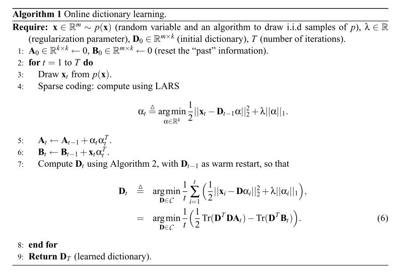
    We propose to replace lines 5 and 6 of Algorithm 1 by:

    $$A_t = \beta_t A_{t-1} + \alpha_t\alpha_t^T$$ $$B_t = \beta_t B_{t-1} + x_t\alpha_t^T$$ $$\beta_t = (1-\frac{1}{t})^\rho$$

    In this circumstance, we propose

    $$D_t = argmin_{D \in C}\frac{1}{\sum_{j=1}^t(j/t)} \sum_{i=1}^t(\frac{i}{t})^\rho(\frac{1}{2}\|x_i-D\alpha_i\|_2^2+\lambda\|\alpha_i\|_1)$$

    =

    $$argmin_{D \in C}\frac{1}{\sum_{j=1}^t(j/t)}(\frac{1}{2}Tr(D^TDA_t)-Tr(D^TB_t))$$

    When $\rho = 0$, we obtain the original version of the algorithm

    In practice, this parameter $\rho$ is only useful for large data sets $(n \ge 100000)$

• 3.4.3 Mini-batch extension

  • The complexity of computing $\eta$ vectors $\alpha_i$ is not linear in $\eta$

  • A Cholesky-based implementation of LARS-Lasso for decomposing one signal has a complexity of $O(kms+ks^2)$, where $s$ is the number of nonzero coefficient

  • When decomposing $\eta$ signals, it is possible to pre-compute the Gram matrix $D^T_tD_t$ and the total complexity becomes $O(k^2m+\eta(km+ks^2))$, which is much cheaper than $\eta$ times the previous complexity when $\eta$ is large enough and $s$ is small

  We propose to replace lines 5 and 6 of Algorithm 1 by:

  $$A_t = A_{t-1} + \frac{1}{\eta}\sum_{i=1}^\eta \alpha_{t,i} \alpha_{t,i}^T$$ $$B_t = B_{t-1} + \frac{1}{\eta}\sum_{i=1}^\eta x_{t,i}\alpha_{t,i}^T$$

• 3.4.4 Slowing down the first iterations

  • Problem:

  The first iterations of our algorithm may update the parameters with large steps, immediately leading to large deviations from the initial dictionary

  • solution:

  Use gradient steps of the form $\frac{a}{b+t}$

  1. $b$ will slow down the first few steps

  2. An initialization of the form $A_0 = t_0I$ and $B_0 = t_0 D_0$ with $t_0 \ge 0$ will also slow down the first steps

• 3.4.5 Puring the dictionary from unused atoms

  • Problem:

  Some of the dictionary atoms are never (or very seldom) used, which typically happens with a very bad initialization

  • solution:

  1. In general cases, replacing these atoms during the optimization by randomly chosen elements of the training set

  2. For more difficult and highly regularized cases, choosing a continuation strategy consisting of starting from an easier, less regularized problem, and gradually increasing $\lambda$

3.5 Link with Second-order Stochastic Gradient Descent

4. Convergence Analysis

5. Extensions to Matrix Factorization

5.1 Using Different Regularizers for $\alpha$

Different priors for the coefficients $\alpha$ may lead to different regularizers $\Psi(\alpha)$

• Positivity constraints on $\alpha$ that are added to the $l_1-regularization$

• The Tikhonov regularization $\Psi(\alpha) = \frac{\lambda_1}{2}|\alpha|_2^2$, which doesn’t lead to sparse solutions

• The elastic net $\Psi(\alpha) = \lambda_1|\alpha|_1 + \frac{\lambda_2}{2}|\alpha|_2^2$

• The group Lasso $\Psi(\alpha) = \sum_{i=1}^s|\alpha|_2$

There is no theoretical convergence results in exploiting non-convex regularizers such as $l_0$ pseduo-norm and $l_p$ pseduo-norm with $p < 1$

5.2 Using Different Constraint Sets for $D$

In dictionary learning, we use an $l_2$-regularization on $D$ by forcing its columns to have less than unit $l_2-norm$, and thus the dictionary update step can be solved efficiently using a block-coordinate descent approach

We can use different convex constraint sets $C′$ as long as the constraints are a union of independent constraints on each column of $D$ and the orthogonal projections of the vectors $u_j$ onto $C′$ can be done efficiently

• The “non-negative” constraints

$$C = \{D \in R^{m * k}\quad s.t. \quad \forall j=1, ... ,k \quad \|d_j\|_2 \le 1 \quad and \quad d_j \ge 0\}$$

• The “elastic-net” constraints

$$C = \{D \in R^{m * k}\quad s.t. \quad \forall j=1, ... ,k \quad \|d_j\|_2^2+\gamma\|d_j\|_1 \le 1\}$$

• Using the $l_1-norm$ only in such problems lead to trivial solutions when $k$ is large enough

• The “fused lasso” constraints

  This kind of regularization has proven to be useful for exploiting genomic data

  $$C = \{D \in R^{m * k}\quad s.t. \quad \forall j=1, ... ,k \quad \|d_j\|_2^2 + \gamma_1\|d_j\|_1 + \gamma_2FL(d_j) \le 1\}$$

  $FL(u) = \sum_{i=2}^m \|u[i]-u[i-1]\|$ which is the $l_1-norm$ of the consecutive differences of $u$

The orthogonal projection onto the “non negative” ball is simple (additional thresholding)

But the projection onto the two other sets is slightly more involved, however they can also be done efficently using some algorithms

5.3 Non Negative Matrix Factorization (NMF)

5.4 Sparse Principal Component Analysis (SPCA)

5.5 Constrained Sparse Coding

5.6 Simultaneous Sparse Coding

6. Experimental Validation

---

• ← Previous Post
• Next Post →